Planar near-rings form a special class of algebraic systems. Here is a short account on the basics of near-rings in general and planar near-rings in particular.
The set of all real functions, together with pointwise addition
and composition, does not form a ring. Observe that
![]() holds by
definition, while
holds by
definition, while
![]() holds for all
holds for all
![]() if and only if
if and only if ![]() is linear, i.e., if
is linear, i.e., if
![]() for all
for all
![]() . Structures of the type like
. Structures of the type like
![]() are
called near-rings:
are
called near-rings:
Of course, every ring is a near-ring; hence near-rings are generalized rings. Two ring axioms are missing: the commutativity of addition and (much more important) the other distributive law.
Actually, the first near-rings considered were
near-fields,
near-rings
![]() in which
in which
![]() forms a group. In 1905,
L. E. Dickson constructed the first proper near-fields by
``distorting'' the multiplication in a field. These types of
near-fields are now called Dickson near-fields. Two years later,
Veblen and Wedderburn used near-fields to coordinatize geometric
planes. In a monumental paper, H. Zassenhaus showed in 1936 that all
finite near-fields are Dickson ones, with the exception of 7
(well-known) cases. 51 years later, Zassenhaus showed that there do
exist non-Dickson infinite near-fields of every prime characteristic.
forms a group. In 1905,
L. E. Dickson constructed the first proper near-fields by
``distorting'' the multiplication in a field. These types of
near-fields are now called Dickson near-fields. Two years later,
Veblen and Wedderburn used near-fields to coordinatize geometric
planes. In a monumental paper, H. Zassenhaus showed in 1936 that all
finite near-fields are Dickson ones, with the exception of 7
(well-known) cases. 51 years later, Zassenhaus showed that there do
exist non-Dickson infinite near-fields of every prime characteristic.
For near-rings, we now have a sophisticated structure theory. Quite
often, the results look similar to the ring case, but the proofs are
completely different. For instance, matrix rings (``the stuff rings
are made of'') have to be replaced by centralizer near-rings
![]() , where
, where ![]() is a fixed-point free automorphism group.
is a fixed-point free automorphism group.
These types of automorphisms turn up in another context as well; this one has nice applications to real-world problems.
This condition is motivated by geometry. It implies that two
``non-parallel lines
![]() and
and
![]() have
exactly one point of intersection''.
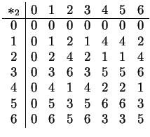
One example is
have
exactly one point of intersection''.
One example is
![]() , where
, where
![]() .
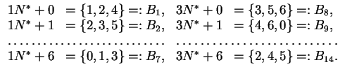
There are various methods to construct
planar
near-rings (see [Cla92,Pil83,Pil96]). Most of them use fixed-point-free
automorphism groups; we just present the easiest way.
.
There are various methods to construct
planar
near-rings (see [Cla92,Pil83,Pil96]). Most of them use fixed-point-free
automorphism groups; we just present the easiest way.
| Field | 1 | 2 | 3 | 4 | 5 | 6 | 7 | 8 | 9 | 10 | 11 | 12 | 13 | 14 |
| Fertilizer | ||||||||||||||
| x | x | x | x | x | x | |||||||||
| x | x | x | x | x | x | |||||||||
| x | x | x | x | x | x | |||||||||
| x | x | x | x | x | x | |||||||||
| x | x | x | x | x | x | |||||||||
| x | x | x | x | x | x | |||||||||
| x | x | x | x | x | x | |||||||||
| Yields: | 2.8 | 6.1 | 1.2 | 8.5 | 8.0 | 3.9 | 7.7 | 5.5 | 4.0 | 10.7 | 3.2 | 4.9 | 3.8 | 5.5 |
The statistical analysis uses the incidence matrix
![]() of the
design:
compute
of the
design:
compute
![]() .
Then Linear Algebra tells us that
.
Then Linear Algebra tells us that
![]() are the best
estimates for the effects of the ingredients
are the best
estimates for the effects of the ingredients
![]() .
In our case, we get the best estimates for the effects of
.
In our case, we get the best estimates for the effects of
![]() as
as
![]() .
If we take
.
If we take
![]() , we can expect a
yield of
, we can expect a
yield of
![]() , which is considerably better than the
yields
, which is considerably better than the
yields ![]() which we got in our experiment. A more detailed
statistical analysis gives confidence intervals for the effects of
which we got in our experiment. A more detailed
statistical analysis gives confidence intervals for the effects of ![]() , as well as information concerning their synergy effects.
, as well as information concerning their synergy effects.
Even more can be done with incidence matrices coming from BIB-Designs.
The rows in the matrix
![]() are
are ![]() -sequences, so they can be
taken as
a binary code
-sequences, so they can be
taken as
a binary code
![]() . This is a nonlinear, constant weight
. This is a nonlinear, constant weight ![]() and constant distance
and constant distance
![]() code of length
code of length ![]() with
with ![]() codewords.
These codes have the largest number of codewords among all codes
with equal weight
codewords.
These codes have the largest number of codewords among all codes
with equal weight ![]() , length
, length ![]() , and fixed minimal distance
, and fixed minimal distance ![]() .
So they also solve discrete sphere packing problems!
.
So they also solve discrete sphere packing problems!